I’ve been working with qdrant since v1.6.0, and maintaining the first qdrant REST API client for .NET (why REST but not gRPC will be evident from this article).
For almost two years I’ve been responsible for qdrant cluster set-up, management, maintenance, query troubleshooting and collection lifetimes.
Today, as I talk about setting up, managing and troubleshooting our own self-hosted qdrant cluster, I invite you to look at the qdrant not from the shiny new vector search algorithms or ML perspective but as a developer tool.
If you are not planning to use self-hosted multi-node qdrant cluster this article might nonetheless be beneficial for you as I will be talking about some qdrant features, not directly related to queries.
For this time I will primarily stick to rectangles and arrows as well as some graphs and configs so no prior C# knowledge is required.
The hardware
So you want your own distributed qdrant cluster, and the perfect place to start is the official qdrant helm chart https://github.com/qdrant/qdrant-helm. It’s perfectly enough to get you up and running, although I found that the support for the recovery mode was limited at the time, so it was added.
Since we use on-premises cluster we have 3 data centers, in 3 logical zones. We have 9 physical nodes split between those zones, each with 112 CPU cores and 374 Gigabytes of RAM. We use 6 nodes for our running cluster and 3 for standby machines (one in each zone) in case one of the machines in production cluster requires maintenance.
This leaves us with the following configuration.
replicaCount: 6

image:
  repository: qdrant/qdrant
  pullPolicy: IfNotPresent
  tag: v1.15.5 # haven't migrated to 1.16 yet as support for 1.16 in our driver is on the way
  useUnprivilegedImage: false # we frequently log in to machines for troubleshooting so we don't use unprivelleged image

args: ["./config/initialize.sh"]
env:
  - name: QDRANT_ALLOW_RECOVERY_MODE # very useful when we need to recover cluster from some critical state
    value: true

resources:
  limits:
    cpu: 106 # maximum cpu available on node (112) - 6cpu for k8s infrastructure and OS
    memory: 370Gi # maximum ram available on node (374) - 4 GB for k8s infrastructure and OS
  requests:
    cpu: 106
    memory: 370Gi
So far so good. Now, before we talk about qdrant nodes configuration let me talk about our collection types.
The collections
We have two main internal customers each of which has its own set of collections. Since the beginning, more than a year ago, we have decided to have all the user’s collections in one physical cluster, although we are planning to split it into per-customer independent clusters to reduce noisy neighbour issues that sometimes arise. Our two main collection types are versioned and live.
Versioned collections
Versioned collections are read-only. They are created, uploaded, indexed, and then no points are added throughout the whole collection lifetime. To make version transition for customer as seamless as possible we utilize an amazing qdrant feature – collection aliases. Each versioned collection name looks like this : public_collection_name~~collection_version , but for the customers the collection is provided under public_collection_name alias.
We initially load data into collections with indexing switched off: the collection is created with hnsw_config.m set to 0. We then load data, and switch M back to the desired number, which kicks the optimizer off. We then await for collection to become ready to switch.
For the sake of data integrity and cluster stability, checking that the collection has Green status is not enough. For collection to function properly and in optimal way we need three things to happen.
- First – all source points should be inserted to the collection. To avoid expensive count operations on not yet ready we compare
points_countto the known number of points in the source data. - Second – we need HNSW index to be present and optimizer to be up and running without issues, as well as have finished merging collection segments. This check is performed by
statusandoptimizer_statuschecks against expected values. We also check segment sizes to be sure that the all segments are merged and we are not left with some unoptimized segments that we have talked about last time. - Third – we need not-empty payload indexes. For these checks we use
payload_schema. We check that indexes have non-zero point counts except the ones that were explicitly allowed to have 0 sizes.
Since there is no single property on the collection info which will tell us all these things have indeed happened, we perform all these checks on timer basis and if all checks succeed we deem collection ready to be switched.
The switching is the easiest part – we just apply an alias public_collection_name to the ready collection. This operation removes an alias form previous version and sets it for the new version. For the user, who always uses public_collection_name , this guarantees a seamless transition to the new version of data.
Live collections
Oddly enough, the versioned collections (think of them as indexed snapshots of data) were the first we’ve implemented. The other type of collection we have is live, i.e. dynamically updated collections. These collections are updated and queried at the same time. They also have a version but they always have the same public name and are not loaded in bulk and switched but rather updated in batches when the new data becomes available.
To make sure that the user queries won’t go to unindexed segments and turn out to be very slow, we utilize params.indexed_only search property to ensure that the engine will only perform search among indexed or small segments.
Node config
Qdrant has several options that can be set upon node startup (and overridden on per-collection basis) via config.yaml. I will show you bits of our setup and tell a little bit about several pitfalls that we have had in the past.
config:
  log_level: DEBUG # yes we grep through debug logs which sometimes give use more insight into problems we encounter
  storage:
    snapshots_config:
      snapshots_storage: s3 # we are currenlty working on snapshot support in our cluster guardian but that's the story for another time.

	# currntly unused but we are planning to experiment with this setting
	update_concurrency: null

  performance:
    # Number of parallel threads used for search operations. Equal to all available CPU.
    # Initially set too high - like several thousands high - which lead to very slow responses on high RPS
    max_search_threads: 106

    optimizer_cpu_budget: 22 # 20% of 106 CPUs. Intially was not set at all which turned out to slow down searches

	  # we are using shard transfers for clearing nodes before removing them from cluster for maintenance
	  # currently we don't change default values but are planning to experiment with them in the future
    incoming_shard_transfers_limit: 1
    outgoing_shard_transfers_limit: 1

  hnsw_index:
    on_disk: false # we always store HNSW and payload in RAM unless explicitly set otherwise per collection

  # found out to be the fastest, obviously. Currently we use shard transfers on versioned collections only so we don't worry about concurrent updates.
  shard_transfer_method: snapshot

  service:
    hardware_reporting: true # as far as I know this feature is still in the preview but we use it anyway for troubleshooting purposes
Now as you have seen the node configuration let’s talk about collection sizes and workloads.
Let’s compare sizes
For the sake of brevity let’s look at three different collection types that we have. We will look at adapted collection info, relevant to our system.
- 25M points sparse vector collection
{
  "collection_name": "sparse_vector_collection",
  "collection_version": "20251117",
  "internal_collection_name": "sparse_vector_collection~~20251117",
  "collection_aliases": [
    "sparse_vector_collection"
  ],
  "is_collection_switched": true,
  "collection_status": "Green",
  "collection_points_count": 25001233,
  "collection_indexed_points_count": 25001233,
  "payload_indexes": [
    "field_1 : Integer : 25001233",
    "field_2 : Integer : 25001233",
    "type : Keyword : 7866787"
  ],
  "on_disk_payload": true,
  "on_disk_hnsw_index": false,
  "default_segment_number": 2,
  "segments_count": 12,
  "max_segment_size_kb": 5000000,
  "sparse_vectors_configuration": {
    "default": {
      "on_disk": false,
      "full_scan_threshold": 1000,
      "vector_data_type": "Float32",
      "modifier": "None"
    }
  }
}
- 20M points 576 vector size quantized collection with more payload indices – this is our customers’ playground for assessing potential benefits different quantization modes can yield
{
  "collection_name": "quantized_binary",
  "collection_version": "20251031",
  "internal_collection_name": "quantized_binary~~20251031",
  "collection_aliases": [
    "quantized_binary"
  ],
  "is_collection_switched": true,
  "collection_status": "Green",
  "collection_points_count": 20073704,
  "collection_indexed_points_count": 20061417,
  "payload_indexes": [
    "field_1 : Integer : 20073704",
    "field_2 : Integer : 20073704",
    "field_3 : Integer : 20073704",
    "field_4 : Integer : 20073704",
    "field_5 : Integer : 20073704",
    "field_6 : Integer : 20073704",
    "field_7 : Keyword : 20073704",
    "id : Integer : 20073704"
  ],
  "on_disk_payload": true,
  "on_disk_hnsw_index": false,
  "default_segment_number": 6,
  "segments_count": 36, // 6 sements per node * 6 shards
  "max_segment_size_kb": 5000000,
  "quantization_settings": {
    "method": "binary",
    "is_store_on_disk": true,
    "encoding": "TwoBits"
  },
  "dense_vector_configuration": {
    "default": {
      "vector_data_type": "Float32",
      "vector_size": 576,
      "vector_distance_metric": "Cosine",
      "hnsw_ef_construct_value": 100,
      "hnsw_m_value": 16,
      "is_store_vectors_on_disk": true
    }
  }
}
- 10M points live collection with relatively small 64 dim vector
{
  "collection_name": "live",
  "collection_version": "20251013",
  "internal_collection_name": "live~~20251013",
  "collection_aliases": [
    "live"
  ],
  "is_collection_switched": true,
  "collection_status": "Green",
  "collection_points_count": 10052364,
  "collection_indexed_points_count": 11183372,
  "payload_indexes": [
    "brand_value_id : Integer : 10052364",
    "camp_ids : Integer : 2496540",
    "local_cate_ids : Integer : 10052364",
    "segment_ids : Keyword : 10047121",
    "seller_admin_seq : Integer : 10052364",
    "ship_to_list : Keyword : 10049302",
    "source_id_item_id : Keyword : 10052364",
    "type : Keyword : 3597024"
  ],
  "on_disk_payload": true,
  "on_disk_hnsw_index": false,
  "default_segment_number": 4,
  "segments_count": 24,
  "max_segment_size_kb": 0,
  "dense_vector_configuration": {
    "default": {
      "vector_data_type": "Float32",
      "vector_size": 64,
      "vector_distance_metric": "Cosine",
      "hnsw_ef_construct_value": 100,
      "hnsw_m_value": 16,
      "is_store_vectors_on_disk": true
    }
  }
}
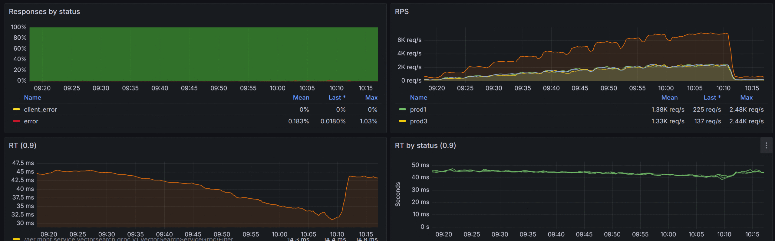
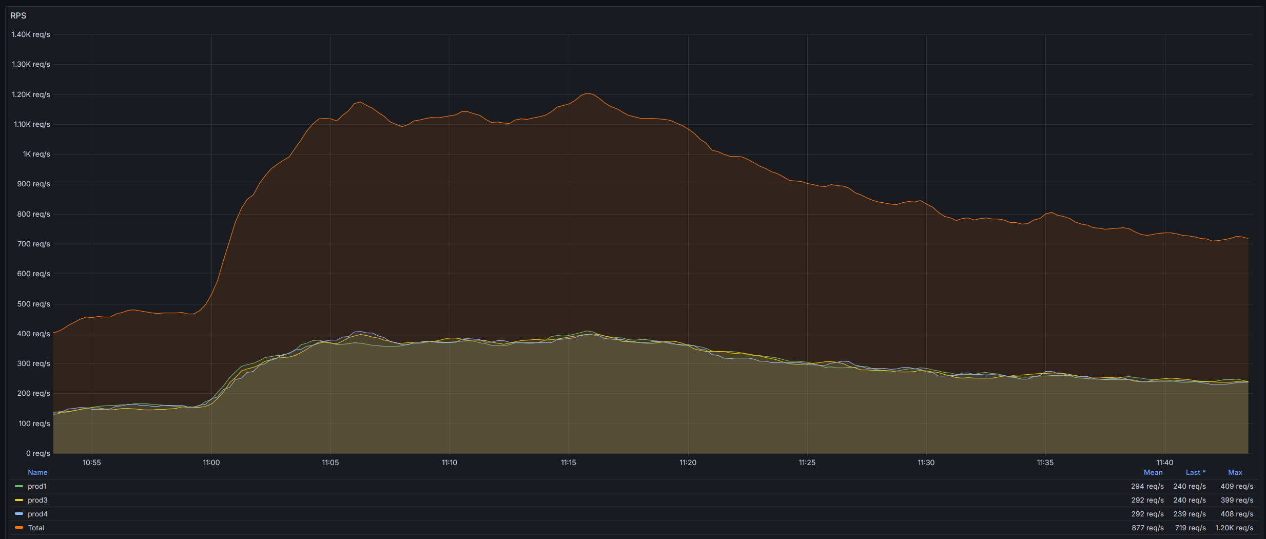
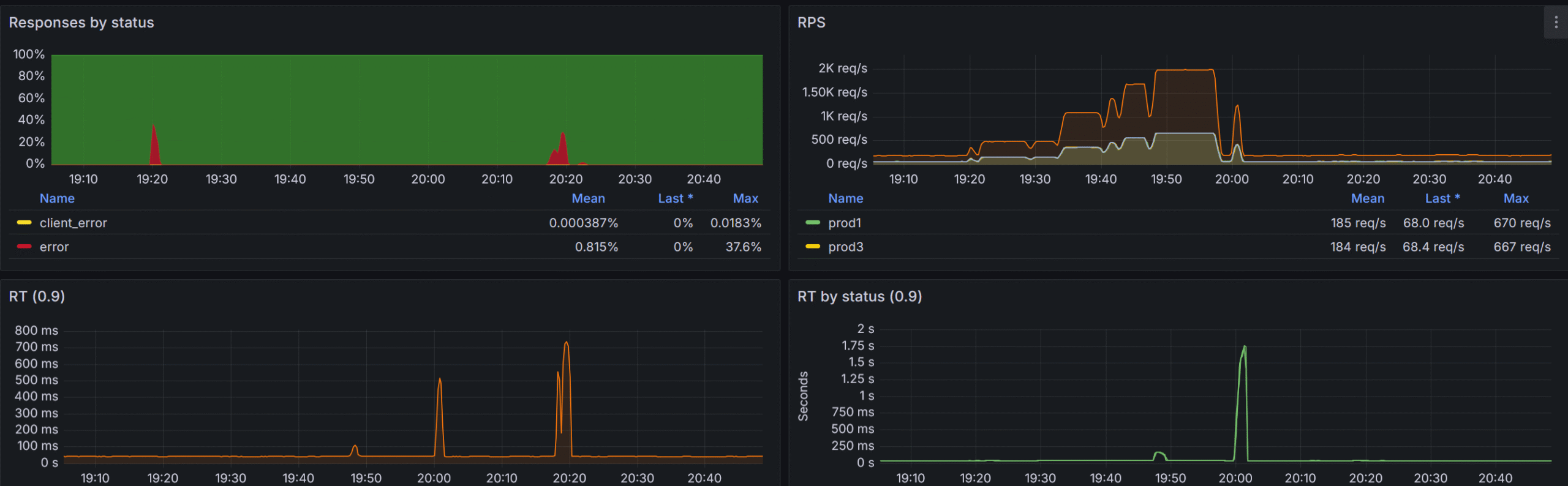
Our peak RPS is 2000 across all the collections with normal RPS of 800-1200. We use a layer of caching implemented via distributed Memcached cluster (be the way check our distributed Memcached library we use for that https://github.com/aliexpressru/memcached) with cache hit ratio of approximately 35%.
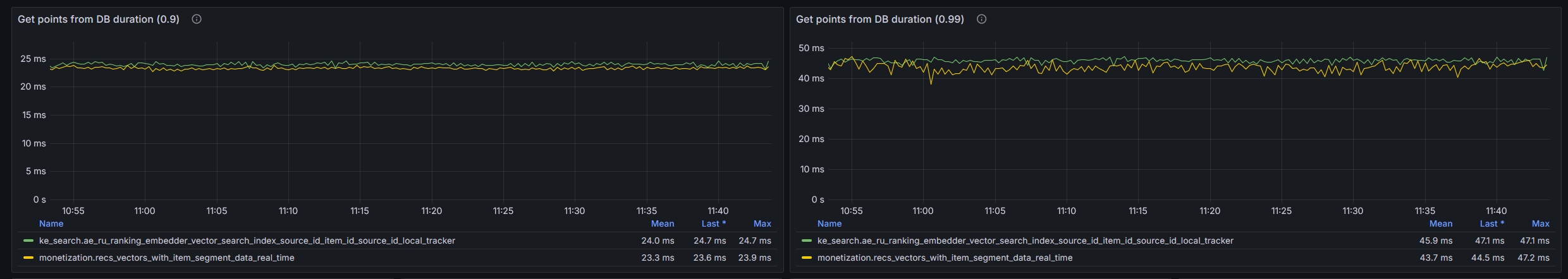
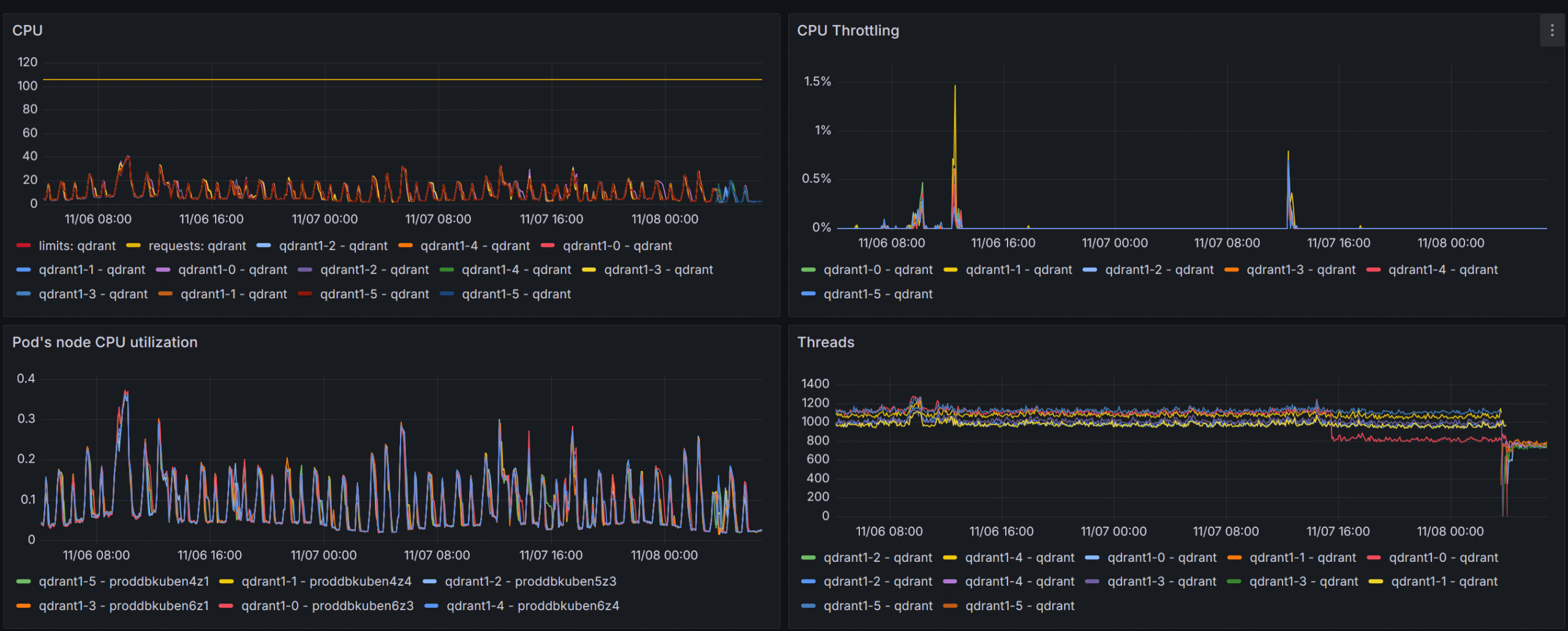
Let’s look at some metrics and then I will talk about the way we achieved that and what problems did we solve on the way.
Problems
Version upload and Query at the same time
Since all the collections live in the same cluster they utilize the same resources both for query and optimization. Thus collection preparation operations may have a negative impact on our query response times.
The first load stage – points insert to the unindexed collection – does not affect response times at all, but when the HNSW index build kicked off, we noticed at least twofold increase in response times.
To mitigate that negative impact we lowered the number of optimization jobs that each collection optimizer was allowed to utilize optimizer_config.max_optimization_threads to 1, while leaving optimization threads in recommended range of 8..16.
{
  "hnsw_config": {
    "max_indexing_threads": 8
  },
  "optimizer_config": {
    "default_segment_number": 2,
    "max_segment_size": 5000000,
    "max_optimization_threads": 1
  }
}
We also set the config.performance.optimizer_cpu_budget for each qdrant node to 20% of the whole available CPU cores. This allowed us to lower the impact almost to 0. At first we resorted to uploading large collections only during quiet night hours but with aforementioned setup is is no longer required.
Insanely high search thread count
At first, before gaining valuable metrics from the qdrant itself (i.e. before adapting the official Grafana board to our setup), the qdrant nodes were set up to have max_serach_threads of 2048 which lead to throttling at RPS > 1000, which, as I understand, was mainly due to context switching in the engine itself.
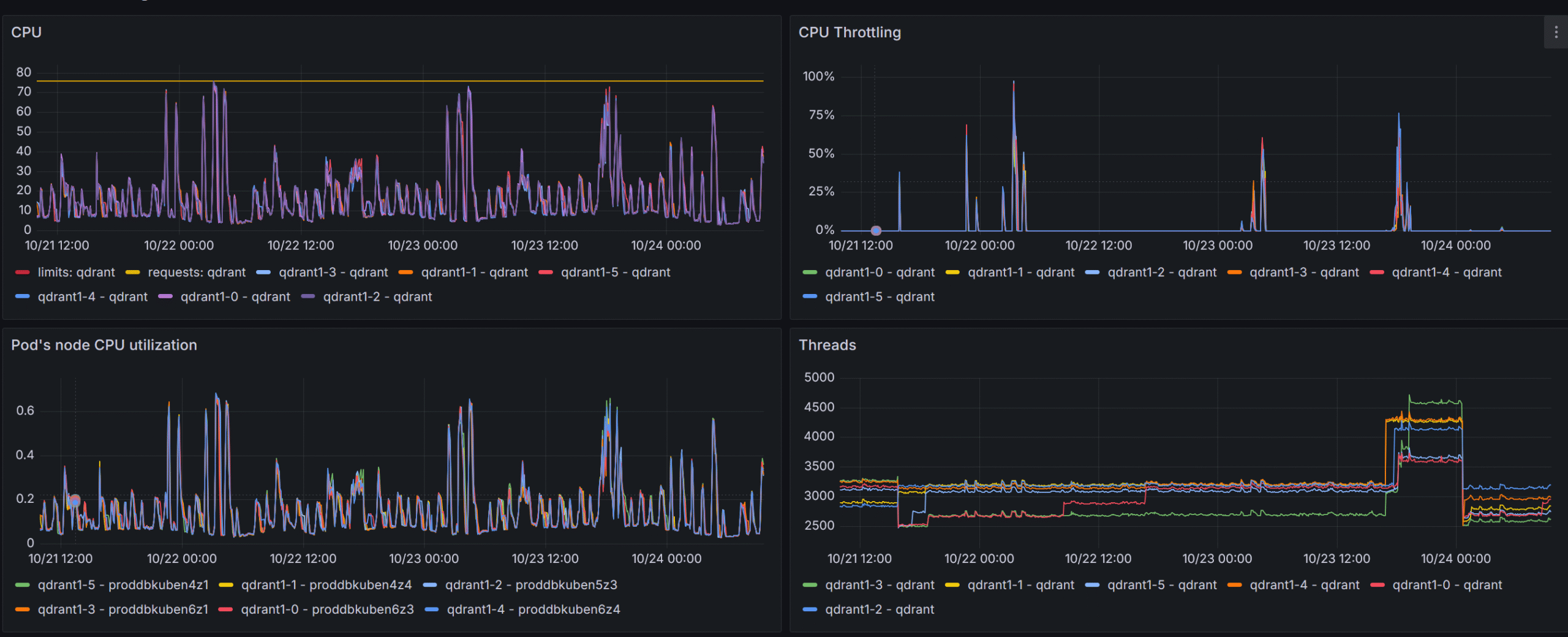
The pain, the suffering!
By lowering the config.performance.max_search_threads on each qdrant node to the number of available cores we completely got rid of that issue.
Invalid filters
As with every database, the user can issue syntactically and logically correct queries that used unindexed payload fields. To make sure that such queries are not reaching the engine the validation system was built in our entry point service. We do not allow customers to issue filters in qdrant syntax, instead we adapt and simplify the filtering system and use that as a template to build qdrant filters ourselves. This way we have more control over the resulting filter.
{
  "filters": [
    {
      "group": "All",
      "operation": "Match",
      "payload_property_name": "field_1",
      "operation_parameters": [
        -1
      ]
    },
    {
      "group": "All",
      "operation": "Match",
      "payload_property_name": "field_2",
      "operation_parameters": [
        "some_value"
      ]
    }
  ]
}
We use filter introspection to walk resulting filter expression, inspect each condition and make sure it uses only indexed fields and – more importantly – uses correct types, i.e. don’t use strings where we expect a number and vice versa. This validation system was build long before the strict mode was implemented (in qdrant 1.13), but currently parts of can be offloaded to qdrant itself, so we are planning to utilize both of these.
Since I have mentioned the driver several times it’s time to see what features it has and how it is different from the official gRPC driver.
.NET driver
Since the very beginning of my journey with qdrant I decided to go with its REST API because it allows cluster management operations which were required since we are brewing our own multi-node cluster. The implementation is mostly trivial with the exception to the filtering system, which was built from ground up (inspired by MongoDB .NET driver). Having full control over the filter structure and request creation also allows us to bypass some inter-version breaking changes – like authorization error codes changing or some response parameters changing places, names and values. This also gives us ability to implement some early filter optimizations like flattening filter layers, and even removing redundant filters and parameters.
But the most benefits of having REST API is that we have full control over the cluster. We can move shards around, work with peers, update cluster setup, get issues information – the operations that are not entirely possible using the official gRPC driver.
In a nutshell we have the following features that differentiate REST API Driver from gRPC one.
- Filter optimization
- Fluent filter building syntax (official driver has some convenience methods to combine conditions but we have gone much further by adding more combination methods as well as some implicit conversions)
QdrantFilter filter =
    Q.Must(
        Q.Must(
            Q<Payload>.MatchValue(p => p.Text, "text_value"),
            Q<Payload>.HaveValuesCount(
                p => p.Array,
                greaterThan: 1,
                greaterThanOrEqual: 12,
                lessThan: 100,
                lessThanOrEqual: 1000
            )
        )
        +
        !Q.MatchValue("key_3", 15.67)
    )
    &
    !(
        Q.Must(
            !Q.MatchValue("key", 123),
            Q<Payload>.MatchFulltext(p => p.Text2, "test_substring"),
        )
        |
        !Q<Payload>.BeInRange(p => p.Int, greaterThanOrEqual: 1, lessThanOrEqual: 100)
);- Shards move and balancing
- Compound cluster operations like draining peer of all collections or redistributing collection shards – all abstracted as one method call
public async Task<ReplicateShardsToPeerResponse> ReplicateShards(
    string sourcePeerUriSelectorString,
    string targetPeerUriSelectorString,
    CancellationToken cancellationToken,
    ShardTransferMethod shardTransferMethod = ShardTransferMethod.Snapshot,
    bool isMoveShards = false,
    string[] collectionNamesToReplicate= null,
    uint[] shardIdsToReplicate = null);

public async Task<DrainPeerResponse> DrainPeer(
    string peerUriSelectorString,
    ShardTransferMethod shardTransferMethod = ShardTransferMethod.Snapshot,
    params string[] collectionNamesToMove);
The next logical step was to have some service that will watch over the cluster and show us some valuable insights into cluster and collection health (unhealthy cluster can have various problems that require multiple parameter analysis) as well as nice GUI to simplify some maintenance features like snapshot creation and recovery.
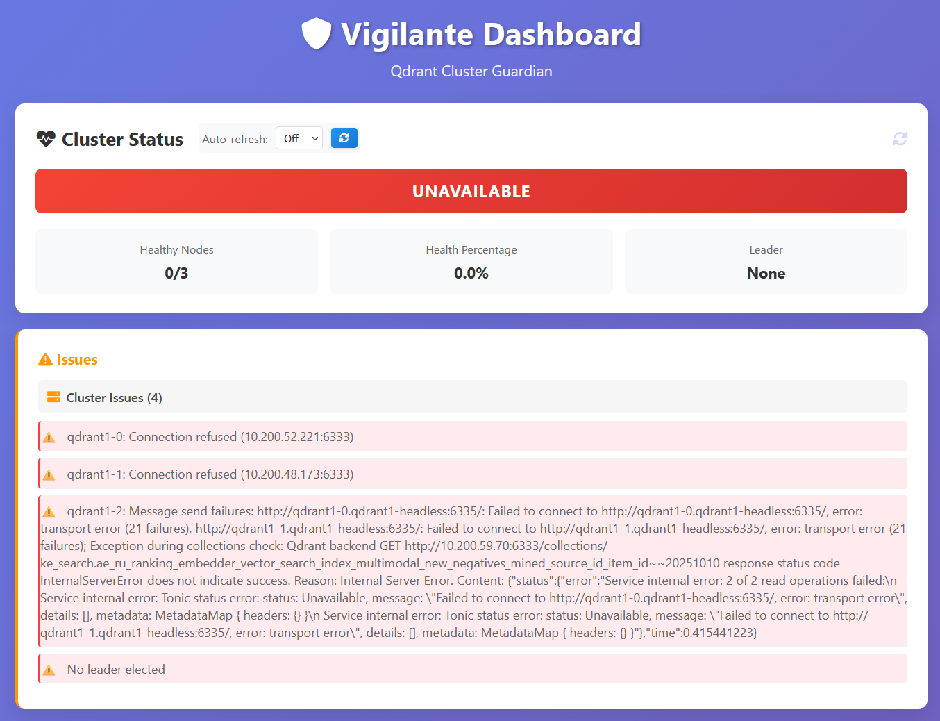
Enter Vigilante
We are currently working on a cluster guardian solution, we call it Vigilante, this solution offers a cluster dashboard with some convenience features available by single button press. I will show screenshots from our 3-node development cluster.
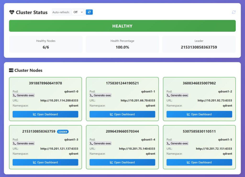
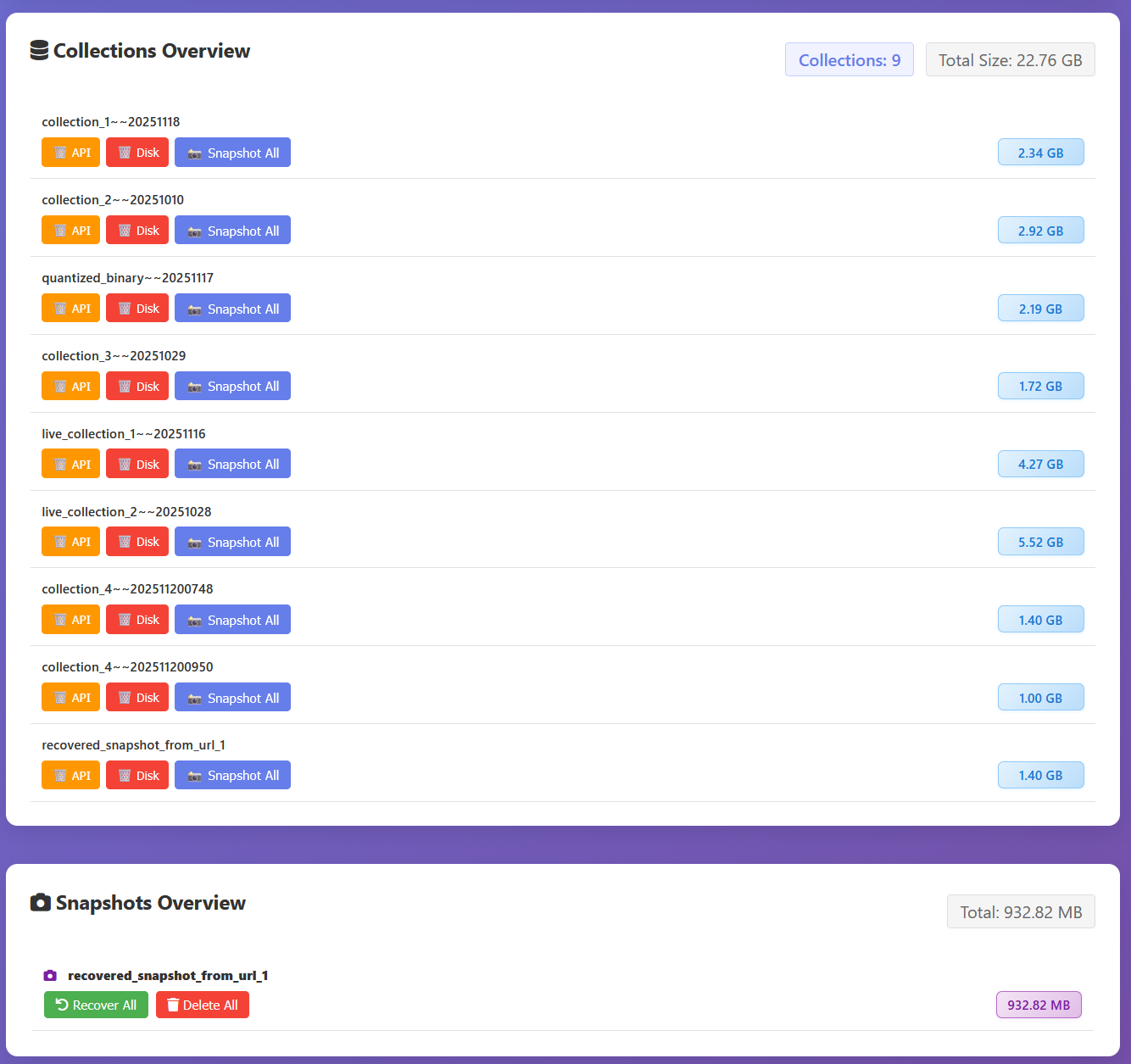
Now let’s look at the unhealthy cluster
We are planning to open-source it in the near future along with our adapted Grafana board – an adaptation of an official board that we use in production – but that’s the story for the next time, so stay tuned.
Final showdown
With all the optimizations and fixes implemented we were able to withstand pretty impressive RPS while keeping our response times as low as 50ms!